
I recently started reading up on how to construct composite high-dynamic-range (HDR) images programmatically. The reason why is because I had been thinking about why traditional cameras have dropped the ball on in-camera HDR when compared to their mobile phone brethren (that’s a thought for another day). There are a number of approaches for building HDR images in computer vision literature. While they differ in how to produce their final output, where they are alike is in their need for the radiometric response function of the imaging pipeline creating the images for the HDR algorithm.
Radiometric response functions describe the mapping of radiance values entering an imaging pipeline to digital pixel values output from an imaging pipeline. With a known response function, the HDR algorithm can output an image with pixel values proportionate to the radiance values as they existed in the scene . Without a known response function, the HDR algorithm must make due with pixel values that do not accurately describe the original scene radiance. This inaccuracy is a feature of response functions. It makes it possible to display high-dynamic-range scenes on standard-dynamic-range displays.
OpenCV provides a CalibrateDebevec class for computing radiometric response functions based on research by Paul E. Debevec. The underlying algorithm is built on the reciprocity property of imaging pipelines.
In an imaging pipeline, the exposure of an image (light energy per unit sensor area) is determined by the sensor irradiance (light power per unit sensor area) multiplied by the exposure time (duration over which the sensor samples data from the scene). The reciprocity property defines that the output of an imaging pipeline is determined by exposure. Thus the same output can be achieved by doubling the irradiance and halving the exposure time (and vice versa). Debevec’s algorithm exploits this property to solve for the original scene radiance values.
The underlying algorithm requires a set of images of a single unchanging scene so that it can make the assumption that the scene’s irradiance in each image is constant. Each image is taken with a different exposure time. With the scene’s irradiance assumed constant and the reciprocity property, the algorithm solves for the irradiance[1] values and radiometric response functions that when plugged into the exposure equations for each image pixel come closest to producing a consensus for pixel values that match those from the set of input images. More specifically, the algorithm minimizes an objective function crafted to satisfy the exposure equations and to account for noise and other image anomalies.
The output of the algorithm is set of relative radiance values, one for each value in the possible set of pixel values for the image format provided to it. For 8-bit images that is one relative radiance value for each of the 256 possible pixel values. For colour images, relative radiance values are produced for each channel.
In preparation for playing with HDR algorithms, I generated a radiometric response function for one of my cameras (an Olympus OM-D E-M5 Mark II) using CalibrateDebevec. The first step was choosing a scene that met the algorithm’s requirements of being static in composition and radiance. I hit both of those requirements by choosing to photograph the laundry closet in my apartment. There there are no windows conveying fluctuating sunlight and no moving objects. The next step was to ensure that the only parameter changing between images was exposure time. To do that I:
- Used the camera’s manual mode. This allowed for fixing the aperture while varying the exposure time.
- Fixed the aperture. I chose f/5.6 as it was a good compromise (on my lens) between light-gathering ability and vignetting levels.
- Fixed the white balance. I calibrated the white balance with a white sheet a paper using the camera’s built-in facility for that (3050K in this case). This avoided changes in white balance between images.
- Fixed the ISO to its base setting. I wanted to avoid the camera’s efforts to improve exposure by varying the ISO to counteract my changes to exposure time.
- Used a tripod. This ensured that the scene was always the same between images.
With the scene and camera setup the next step was to capture the images. There are two considerations for this step:
- The number of images
- The exposure time for each image
Debevec’s paper gives a guideline for choosing the number of images:
N(P – 1) > (Zmax – Zmin)
Where N is the number of pixels sampled in each image, P is the number of images, and (Zmax – Zmin) is the maximum pixel value range for your image pipeline. For an 8-bit image (range of 255) and CalibrateDebevec’s default of 70 pixels sampled, a minimum of 4 images are required. More images can be added depending on how wide the dynamic range of the scene is. I used 16 images matching the amount used in Debevec’s paper (exposures available in the OpenCV repository).
The paper also provides a guideline for choosing exposure times. The exposure times must be unique per image but must also be similar enough that some pixels fall in the working range for the imaging pipeline’s response in multiple (adjacent) images. The working range of the response being the middle region of the response curve where large changes in radiance produce large changes in pixel values i.e. the imaging pipeline’s most sensitive region. This ensures that the algorithm has enough information to relate images to each other. I chose the same exposure time selection used in Debevec’s paper:
| Inverse Exposure Time | On-Camera Exposure Time |
| 0.03125 | 32 |
| 0.0625 | 16 |
| 0.125 | 8 |
| 0.25 | 4 |
| 0.5 | 2 |
| 1 | 1 |
| 2 | 1/2 |
| 4 | 1/4 |
| 8 | 1/8 |
| 16 | 1/16 |
| 32 | 1/32 |
| 64 | 1/64 |
| 128 | 1/128 |
| 256 | 1/256 |
| 512 | 1/512 |
| 1024 | 1/1024 |
With images in-hand the next step is to process those images using OpenCV. I used the code below which follows the example laid out in the OpenCV documentation:
| #include <fstream> | |
| #include <iostream> | |
| #include <opencv2/core/utility.hpp> | |
| #include <opencv2/imgcodecs.hpp> | |
| #include <opencv2/photo.hpp> | |
| void load_exposure_data(std::ifstream& list_file, | |
| std::vector<cv::Mat>& exposures, | |
| std::vector<float>& exposure_times); | |
| bool response_monotonic(const cv::Mat& response); | |
| void write_response_csv(std::ofstream& csv, const cv::Mat& response); | |
| int main(int argc, const char* argv[]) { | |
| const std::string keys{ | |
| "{l list |list.txt| list file of images and inverse exposure times}" | |
| "{o output |response.csv| file path at which to save response CSV}"}; | |
| cv::CommandLineParser parser(argc, argv, keys); | |
| std::string list_file_name{parser.get<std::string>("list")}; | |
| std::ifstream list_file(list_file_name); | |
| std::vector<cv::Mat> exposures; | |
| std::vector<float> exposure_times; | |
| load_exposure_data(list_file, exposures, exposure_times); | |
| std::cout << "Loaded exposure data from: " << list_file_name << "\n"; | |
| cv::Ptr<cv::CalibrateDebevec> calibrator = cv::createCalibrateDebevec(); | |
| cv::Mat response; | |
| calibrator->process(exposures, response, exposure_times); | |
| if (response_monotonic(response)) { | |
| std::cout << "Calculated response is monotonic.\n"; | |
| } else { | |
| std::cout << "Calculated response is not monotonic.\n"; | |
| } | |
| std::string output_file_name{parser.get<std::string>("output")}; | |
| std::ofstream csv(output_file_name); | |
| write_response_csv(csv, response); | |
| std::cout << "Wrote response to: " << output_file_name << "\n"; | |
| return 0; | |
| } | |
| void load_exposure_data(std::ifstream& list_file, | |
| std::vector<cv::Mat>& exposures, | |
| std::vector<float>& exposure_times) { | |
| std::string exposure_file_name; | |
| float inverse_exposure_time; | |
| while (list_file >> exposure_file_name >> inverse_exposure_time) { | |
| cv::Mat exposure{cv::imread(exposure_file_name)}; | |
| exposures.push_back(exposure); | |
| exposure_times.push_back(1 / inverse_exposure_time); | |
| } | |
| list_file.close(); | |
| } | |
| bool response_monotonic(const cv::Mat& response) { | |
| bool at_start{true}, is_monotonic{true}; | |
| float blue_before{0}, green_before{0}, red_before{0}; | |
| cv::MatConstIterator_<cv::Vec3f> response_iter{response.begin<cv::Vec3f>()}; | |
| for (; response_iter != response.end<cv::Vec3f>(); ++response_iter) { | |
| float blue_now{(*response_iter)[0]}, green_now{(*response_iter)[1]}, | |
| red_now{(*response_iter)[2]}; | |
| if (at_start) { | |
| blue_now = blue_before; | |
| green_now = green_before; | |
| red_now = red_before; | |
| at_start = false; | |
| continue; | |
| } | |
| if (!(blue_before <= blue_now || green_before <= green_now || | |
| red_before <= red_now)) { | |
| std::cout << blue_before << blue_now << green_before << green_now | |
| << red_before << red_now; | |
| is_monotonic = false; | |
| break; | |
| } | |
| } | |
| return is_monotonic; | |
| } | |
| void write_response_csv(std::ofstream& csv, const cv::Mat& response) { | |
| csv << "blue_input,blue_response,green_input,green_response," | |
| "red_input,red_response\n"; | |
| int pixel_value{0}; | |
| cv::MatConstIterator_<cv::Vec3f> response_iter = response.begin<cv::Vec3f>(); | |
| for (; response_iter != response.end<cv::Vec3f>(); ++response_iter) { | |
| csv << (*response_iter)[0] << "," << pixel_value << "," | |
| << (*response_iter)[1] << "," << pixel_value << "," | |
| << (*response_iter)[2] << "," << pixel_value << "\n"; | |
| ++pixel_value; | |
| } | |
| csv.close(); | |
| } |
The code loads image file names and their associated exposure times from a file. It then opens the images and feeds the image data and exposure times to CalibrateDebevec for processing. The responses output by CalibrateDebevec can then be output to a CSV where they can be loaded into a spreadsheet for visualization:
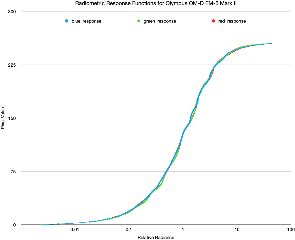
When visualized one can see that the responses differ for each colour channel. One can also see colour detail in the lower region of relative radiance is sacrificed for detail in the upper region.
From here I will be generating responses for other cameras that I have. Namely a Canon EOS Rebel SL1 (26-08-2020: responses generated) that I will be using with Canon’s SDK and OpenCV. After that is a dive into HDR algorithms to explore what is possible with the current state of the art.
[1] We started out solving for radiance to pixel mappings. Why the switch to irradiance here? Irradiance is proportional to radiance and that proportionality can be assumed constant across a sensor for apertures of f/8 and smaller. Thus the terms are interchangeable provided that aperture requirements are met.

One thought on “Radiometric Response Functions in OpenCV”